When you go back home in the cold winter, you may like to turn on the air conditioner or heater immediately and hope it becomes warmer as soon as possible. We notice that we feel warmer when we get close to the heater, and the bigger the space, the temperature will take longer increase.
Given a certain condition, the heat equation can be used to find the temperature at any point at any time. However, the heat equation is hard to understand for people without a mathematical background.
We can imagine an empty space as a 3D grid and heat energy as ‘tiny’ heat particles. Given an initial temperature in the space and a boundary condition, the heat transfer process can be simulated by letting all heat particles move to one of their nearest neighbouring points with probability 1/8 at each short time step.
The temperature at a certain point at any time is equal to the density of heat particles at that point at that time.
The simulation can be extended to other dimensions of mathematical integer lattice, for example, one dimensional case for the heat transfer in a steel rod. A particle making a random move to an adjacent point, where the probability for which adjacent point is equal, is known as simple random walk in integer lattice.
As a result, the heat equation can be interpreted in the probabilistic way, and it resembles the random walk. Probability adds an extra view in terms of movements of individual random particles. This extra view is useful for understanding the equation.
In the continuous space and continuous time, the heat equation can be interpreted with the Brownian motion. Brownian motion can be imagined as the limit of a random walk with very small steps.
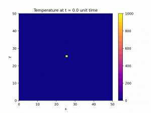
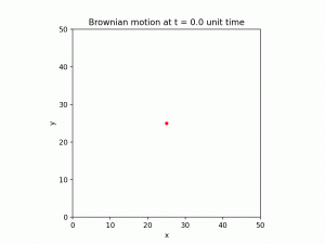
The following two GIF present the simulation of heat transfer when there is initially a large amount of heat energy in the middle of the 2D space. The left GIF shows the result of heat equation, and the right GIF shows the particles doing Brownian motion.
Huan Chen
Monash University


